Figure 3.1. Comparison between 2K and 4K resolution.
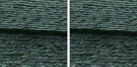
Both images are enlarged portions scaled to the same size. The 4K image on the right hand side displays more visible details and appears to be sharper than the 2K image on the left. Although, viewed in a projection, the differences may be less noticeable.
Figure 3.2. Aliasing in digital image.
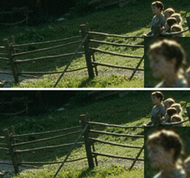
Both images were down-sampled from a higher resolution. To make the effect more visible, an enlarged portion is shown. A proper digital filter was used for the upper image and it does not show aliasing. In the lower image no filtering was applied producing an edgy structure in the diagonal lines. Aliasing can also increase the noise or grain in an image as shown in the enlarged face.
In scanning, the original film image would represent the higher resolution image that is sampled at a lower rate. Without filtering similar effects could occur.
Figure 3.3. Grayscale gradient in different bit depths.

The upper grayscale is encoded in 8 bits, which gives 256 levels. more than the eye can differentiate. With each bit less the number of levels is halved. The visual effect seen in the lower bit depths is called banding or contouring. You may have to view the full size version of the image to see the effect.
Figure 3.4. Color processing in different bit depths.

Digital scans stand at the beginning of the post production process. Color processing may make banding visible where the tonal variation of the original image appears to be smooth. The image color gradient on the left hand side is the original image in this example. It is manipulated with some typical tools in digital color correction (gradation curves). The second image shows the result of a 16 bit processing, while the last image is the result of the same process carried out in 8 bit.
Figure 3.5. Encoding of negative densities in the Cineon/DPX file format.
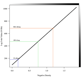
The DPX file is simply a linear encoding of negative densities. See Table 3.1 for the code values of the marked points.
Figure 3.6. Scene in log density encoding.
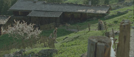
This is the DPX scan that was used to produce Figure 1.1. It is displayed as it is, without gamma correction.
Figure 3.7. Specific tonal values in the sample image.
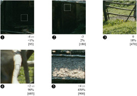
The numbers display the relative log exposure in stops (top line), the relative linear exposure, and, in the bottom line, the resulting code value in a Cineon/DPX scan of the negative.
Figure 3.8. The histogram of the log encoded sample image.
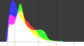
The number of pixels towards the minimum and maximum code values is zero. The range of tonal values is continuous without gaps.
Figure 3.9. Histogram showing gaps.

This is an artificially produced example. A histogram of a color corrected image may show gaps, but the raw scan should have a continuous variation of tonal values.
Figure 3.10. Relation between film transmittance and sensor signal.
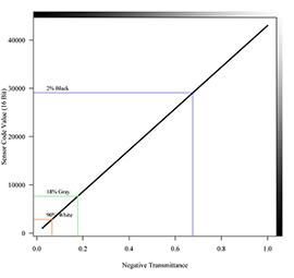
The digital image sensor in a scanner “sees“ the transmittance of the negative. Note that the transmittance decreases with the exposure.
Figure 3.11. Relation between sensor signal and log encoding.
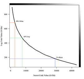
A sensor with more than 14 bit quantization is needed to produce the desired resolution of 1/500 log D over the entire density range.
Figure 3.12. Scene in linear luminance encoding (full range).
The image is gamma corrected for display on a monitor, otherwise it would appear even darker.
Figure 3.13. Linear encoding of scene luminance in 16 bit code values.
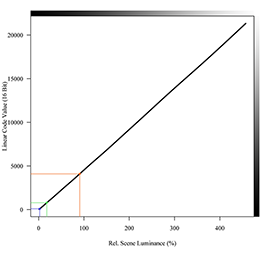
The 90% white point is mapped to 1/16 of the maximum code value giving the headroom that is needed to represent the highlights.
Figure 3.14. Encoding of log scene luminance in 10 bit code values.
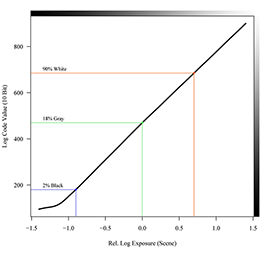
Since the DPX file is a linear encoding of negative densities, it is also a linear encoding of log scene luminance.
Figure 3.15. Relation between scene luminance and scanner sensor signal.
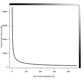
The sensor code values represent transmittance of negative film, which is not linearly related to scene luminance.
Scanning resolution is one key issue when it comes to scanner performance. Many tests and demonstrations have been done to show the ultimate resolution of film. Most scanning is currently carried out at 2K resolution, i.e. the image is sampled with 2048 pixels per line. For comparison, HDTV has 1920 pixels per line. 4K (4096 pixels per line) scans are sometimes performed for VFX, and some productions, Spider Man 2 for example, have been done entirely in this format. Looking at the digital files in Figure 3.1, a 4K scan definitely contains more details than a 2K scan. The trade-offs are scanning time per frame, data transfer times, and processing costs.
Care needs to taken that no aliasing appears in the scans. In digital imaging, aliasing is a term used when patterns are created in an image that were not in the original. It can be avoided by resampling to a lower spatial resolution with a digital filter or by an optical filter. Optical anti-aliasing filter, however, tend to produce less sharp images.
Dynamic range is the other key issue, meaning the scanner needs to capture the entire density range of the negative. Even though this may contain information that will not be shown in the final image, it gives headroom to change the dynamics of a shot to fit creative requirements.
Together with dynamic range comes the question of quantization. A scanner has to translate the continuous range of densities in a negative into discrete digital numbers. The bit depth or number of bits per channel determines how many levels can be encoded. Usage of 8 bits results in 256 levels, a number generally considered too low for negative film scanning. One needs more than 100 levels to produce a perfectly smooth tonal scale. Lower quantization breaks graduated colors into visible blocks. The effect is called banding or contouring and is illustrated in Figure 3.3 and Figure 3.4. Color processing may make banding visible where the tonal variation of the original image appears to be smooth. Therefore, scans with a higher bit depth than 8 bits are needed as source for the color correction.
A commonly used file format for film scans is the Cineon or DPX format. It uses 10 bits per channel, which equals 1024 levels, and linearly encodes the densities of the negative above base as shown in Figure 3.5. One code value in the DPX file represents 1/500 log D. A look at Table 3.1 reveals that the base density of the negative is encoded as 95 rather than zero. That happens for the same reason an IN is about 0.2 log D heavier than the original negative (see the section called “Characteristic Curve”). Recording the Cineon image on intermediate film results in a digital IN, where the densities are shifted by 0.19 log D. More information about the Cineon and DPX format is given in the appendix.
Figure 3.6 displays the sample image in log encoding. Figure 3.7 shows 5 enlarged portions of the image together with the code values from the scan of the negative. A DPX file presents a positive image but otherwise it keeps the characteristic of a negative. One could regard it as the digital version of an interpositive. It looks “flat”, the blacks are too high, and the whites are to low since the additional tonal values below and above are linearly encoded as well. Like film negatives, Cineon/DPX images are not meant to be judged by the human eye.
Nevertheless, a scanner operator or colorist has to examine the scans. Since a film scanner applies no color correction, the scan may not look neutral. The midtones may not necessarily sit around a code value of 470 because some cinematographers prefer to overexpose the negative by one or two stops. Examine the histogram in Figure 3.8. It shows the relative frequency of the code values in the sample image. The number of pixels towards the lower and upper limit of the range is zero. A DPX image with a significant number of pixels having a value of 0 or 1023 is most likely the result of a misalignment of the scanner. Also, there should be no gaps in the histogram. Natural images always have a continuous variation of tonal values. Remember to display the histogram 1024 pixels wide to recognize any gaps. Figure 3.9 gives an example of a histogram showing missing code values in the higher densities.
Table 3.1. Relation of negative densities and 10 bit log code values.
| Label | Density Above Base | Log Code Value (10 Bit) |
|---|---|---|
| D-Min[1] | 0.00 | 95 |
| 0.01 | 102 | |
| 0.02 | 107 | |
| 0.05 | 122 | |
| 0.11 | 151 | |
| 2% Gray [2] | 0.17 | 180 |
| 0.23 | 212 | |
| 0.30 | 244 | |
| 0.36 | 277 | |
| 0.43 | 309 | |
| 0.49 | 341 | |
| 0.56 | 373 | |
| 0.62 | 406 | |
| 0.69 | 438 | |
| 18% Gray [3] | 0.75 | 470 |
| 0.81 | 501 | |
| 0.87 | 531 | |
| 0.93 | 562 | |
| 1.00 | 593 | |
| 1.06 | 624 | |
| 1.12 | 654 | |
| 90% White [4] | 1.18 | 685 |
| 1.24 | 716 | |
| 1.30 | 746 | |
| 1.36 | 777 | |
| 1.43 | 808 | |
| 1.49 | 839 | |
| 1.55 | 869 | |
| D-Max [5] | 1.61 | 900 |
| 1.67 | 931 | |
| 1.73 | 961 | |
| 1.79 | 992 | |
| 1.86 | 1023 |
Each line in the table corresponds to an exposure increment of one third stop. The numbers in the column titled “Label“ refer to the markers in Figure 1.1. Enlarged portions of the marked areas are displayed in Figure 3.7.
An important precondition for correctly scanning a negative is the base calibration of the scanner. The intensity of the light source in the scanner must be adjusted accordingly to the density of the clear base of the film. Otherwise, parts of the information in the shadows (if the light intensity is too high) or in the highlights (if the light intensity is too low) could be lost in the scan.
DPX code value = 95 + 500 * density above base
density above base = DPX code value / 500 - 0.19
Most film scanners use a CCD (charge coupled device) or a CMOS (complementary metal oxide semiconductor) element as image sensor. Both types of imagers convert light into electric charge and process it into electronic signals. The response of both sensors is related to the transmittance of the film. However, the important photographic quantity is the density.
Although one can easily convert transmittance to density, there is a difficulty. The conversion function is very steep at high opacity/density values, as shown in Figure 3.11. Therefore, more code values or more bits are needed in the sensor output than in the final file format, the film transmittance must be sampled with a higher quantization than the density.
Some people prefer to work with linearly encoded images instead of the Cineon/DPX format. Confusingly, there are at least three different types of encoding referred to as “linear”.
-
Video images which can be properly displayed on a video monitor without any additional transformation. Video images are not linear, however. First, they need to be gamma corrected as will be explained in Section 5.1. Second, one must introduce some shadow and highlight compression to display a natural scene on a monitor.
-
A linear encoding of the (linear) scene luminance. One can invert the characteristic curve of a negative assuming normal exposure and an average film gamma of 0.6 (the formula is given below). While this encoding is useful for integration of computer rendered elements, it is, like DPX images, not easily viewable. Figure 3.13 shows the placement of the reference tonal values. The white point is mapped at 1/16 of the maximum code value and accordingly, the image in Figure 3.12 looks much too dark if displayed without any further means of correction. Since most of the code values are used to record the highlight information, a linear image needs more bits to produce the same detailed shadow representation as a log encoded image.
-
Some scanners, the ARRISCAN for example, allow one to save the linear sensor image. Looking at Figure 3.15, one sees the code values are not linearly related to the scene luminance because they represent the transmittance of negative film.
Although it is not regarded as “linear” the DPX format is actually a linear representation of log scene luminance, compare Figure 3.13 with Figure 3.14.
relative luminance = 10 ^ ( (dpx code value – white point) * 0.002 * negative gamma )
Commonly, the negative gamma is assumed to be 0.6 and the white point is set to 685.
The result is relative luminance where the reference white is placed at 1.0. To convert into a format like 16 bit TIFF the luminance values are multiplied by 4095 leaving a headroom of 4 stops for the highlights. The resulting transfer curve is displayed in Figure 3.13 and Figure 3.12 shows the sample image in this encoding.
Figure 3.16. Low and high image used in the ARRISCAN
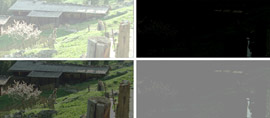
The upper right image is scanned with ten times more light than the image on the left hand side. (If you are thinking the order is reversed, remember that a negative image is scanned.) The left image is shifted down by the equivalent of 1.0 log D, while the right image is shifted up. The resulting images in the second row are combined into one.
The ARRISCAN was introduced in 2004 and shows several features distinguishing it from other film scanners.
-
Pin registered transport with full frame sensor. During the image exposure film, gate, and sensor are locked into position. This results in high stability and consistency.
-
High dynamic range by combining a low and a high frame. The scanner takes two exposures per channel. The first one (Figure 3.16 left hand side) captures the negative densities up to 1.0 log D. The second one (Figure 3.16 right hand side) is done with 10 times more light and captures the densities above 1.0.
-
LED illumination. LED’s have a much longer durability than the Xenon or HMI lamps used in other scanners. Also their color stays constant during the entire life cycle. Another advantage is that the LED illumination produces almost no heat in the film gate.
-
Oversampling. The final 2K or 4K image is produced from a 3K respectively 6K scan to avoid aliasing.
-
High speed scanning with four frames per second in 2K (will be released at IBC 2005).
-
The widely used Cineon/DPX image file format is a linear representation of negative densities and is therefore linear to log scene luminance measured in log exposure or stops.
-
Image formats with a linear encoding of linear scene luminance need a higher bit depth.
-
A scanner sees neither film densities nor scene luminance, it sees film transmittance which has to be converted to a photographic meaningful metric. Because of this conversion the internal bit depth needs to be higher than the output bit depth.
-
A scanner should scan with a higher spatial resolution than the output format to avoid aliasing.